The kinematic equations describe the motion of an object in classical mechanics. In the simple case of uniformly accelerated motion in one dimension, they provide us with useful results for relating the variables involved. These variables include velocity (v), time (t), acceleration (a) and displacements (s) of the object.
So, let us look at the four kinematic equations.
Index
Velocity – Time Relation
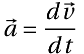
This relation can be obtained from the definition of acceleration:
In the case of uniform acceleration in one dimension, this reduces to:
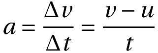
Where
v is the final velocity
u is the initial velocity
Δt is the time interval.
If we take the initial time as 0, we can just write Δt = t as done above
Thus, by rearranging terms, we obtain the first kinematic equation:
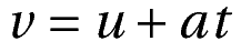
This kinematic equation is the velocity-time relation.
Example: If a particle, starting at u = 2 m s-1 accelerates at a = 0.1 m s-2 for t = 20 s, What will be its final velocity?
Applying the velocity-time relation, we get that its final velocity
v = 2 + (0.1)(20)
=> 2 + 2
=> 4 m s-1
Displacement – Velocity Relation (With Time)
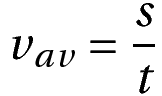
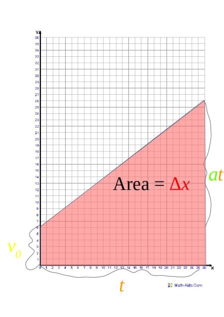
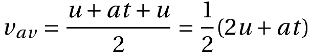
The average velocity vav is just a time-averaged value of the object’s velocity at various times. The average velocity formula is as follows:
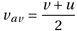
In the case of uniformly accelerated motion in one dimension, the average velocity has a simple formula. It is equal to half of the sum of the initial velocity (u) and final velocity (v).
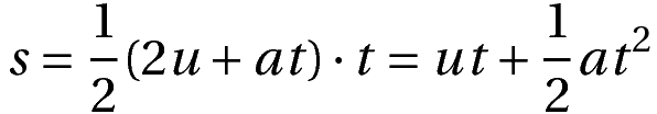
Using the above two equations, we get the result:
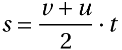
This kinematic equation is the relationship between displacement and velocity, with time present.
Example: Consider a particle that starts with velocity u = 3 m s-1 and has final velocity v = 1 m s-1. If it travels for t = 30 s, What is the displacement?
The displacement s covered in the time is
= (3+1/2)(30)
=> 60 m.
Displacement – Time Relation
If we substitute the results of the velocity-time relation in the expression for average velocity, we can get rid of final velocity v.
Then, if we substitute this in the previous relation for velocity and displacement, we obtain:
This kinematic equation is the relation between displacement and time.
Example: Consider an object accelerating at a = -10 m s-2 for t = 5 s. Let its initial velocity u = 0. What is the distance travelled?
The equation gives us that the distance travelled is
=> s = (0)(5)+(0.5)(-10)(5^2) = -125 m.
Note that the negative sign indicates that the displacement is opposite to the chosen positive axis. This example can be of an object in free fall due to gravity for 5 s.
Displacement – Velocity Relation (Without Time)
We can get rid of time in the displacement-velocity relation. For this, note that time can be written as:
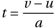
Now we eliminate time by substituting the above in the previous displacement – velocity relation. This gives us:
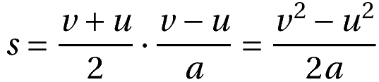
This result is often stated as
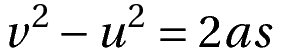
This kinematic equation is the displacement-velocity relation.
Example: Consider a car with initial velocity 20 m s-1 and final velocity 0 m s-1. Let it come to rest in a distance s = 200 m. What is the acceleration?
We can then calculate the acceleration as a = (02 – 202)/200 = – 2 m s-2.
Uses
The kinematic equations have a wide variety of uses in cases where a particle accelerates at a uniform rate. In classical mechanics, this is equivalent to the case where the particle is acted upon by a constant force. A common case where this can be used is in studying a freely falling object.
Further, we can extend these equations to higher dimensions, if we take suitable components of velocity, acceleration and so on.