The Navier Stokes Equation is one of the most important partial differential equations in fluid dynamics. It can be used to describe the motion of any fluid in space.
It is a part of the Millenium Prize Problems, which is a group of seven problems in mathematics that were stated by the Clay Mathematics Institute on May 24, 2000.
Until around 1822-23, all theoretical developments with regard to the motion of fluids considered them to be ideal, and without viscosity. This had been the case since the publication of Euler’s equation of motion for non-viscous fluids since 1755. But, the idea existed that the reason for the deviation of experimental results from theory was due to viscosity.
Despite this, very few attempts were made to obtain an equation of motion which took viscosity into account. This was finally done successfully by Navier in 1823.
Index
Assumptions Made
To explain the Navier Stokes Equation below, the following assumptions are made:
- The fluid used is Newtonian: A Newtonian fluid’s viscosity remains constant, no matter the amount of shear applied for a constant temperature. These fluids have a linear relationship between viscosity and shear stress.

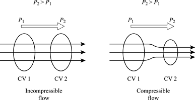
- The fluid used is Incompressible: An incompressible fluid is a fluid whose density does not change when the pressure changes. There is no real incompressible fluid, this is an ideal condition.
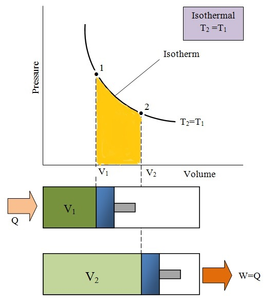
- The process is Isothermal: An isothermal process is a change of a system, in which the temperature remains constant. That is, ΔT = 0.
A Note on the Mathematics Used
Here, we look at a couple of mathematical terms/operators used to describe the Navier Stokes equations.
Divergence
In vector calculus, divergence is a vector operator that operates on a vector field, producing a scalar field giving the quantity of the vector field’s source at each point. More technically, the divergence represents the volume density of the outward flux of a vector field from an infinitesimal volume around a given point.
For a vector v, the divergence is denoted by:
div(? ) = ∇ · ?
In physical terms, the divergence of a vector field is the extent to which the vector field flux behaves like a source at a given point.

.svg)
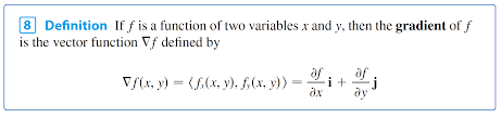
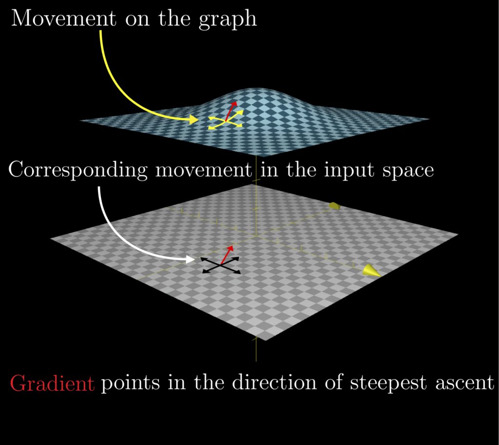
Gradient
The gradient of a function v, denoted as ??, is the collection of all its partial derivatives into a vector.
The gradient is a fancy word for a derivative or the rate of change of a function. It’s a vector (a direction to move) that points in the direction of greatest increase of a function.
Laplace Operator
In mathematics, the Laplace operator or Laplacian is a differential operator given by the divergence of the gradient of a function on Euclidean space. For a vector v, the Laplace Operator is denoted by ∇.∇.v, or ∇2?.
The Navier Stokes Equations Explained
The Navier Stokes equations consist of two equations, both of which are based on basic principles of physics. The two equations are:
- ∇ ⋅ ? = 0
- ρ (d?/dt) = -∇p + μ∇2u + F
where:
? = Velocity of fluid (Vector Field)
ρ = Density of fluid
∇p = force due to Pressure gradient
μ∇2u= Friction/viscosity component
F = external forces acting on the fluid
We will quickly talk about each of the equations individually.
Let us start with equation 1:
∇? = 0
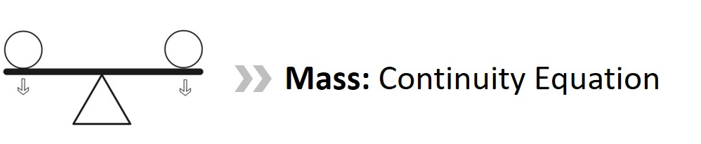
This equation tells us that mass is conserved within the fluid. The operator used here is the divergence, and the vector field, in this case, is the velocity vector field of the fluid ?.
From the discussion of divergence earlier, we know that the operator is used to describe how much or how little a point acts as a source for the fluid. The existence of source or sink implies that some of the fluid simply vanishes, hence zero divergence implies that the mass is conserved.
Equation 2 is given by:
ρ (d?/dt) = -∇p + μ∇2u + F
This is just a version of Newton’s second law, which is given by:
ma = ΣF
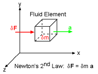
Let us quickly look at how the second Navier Stokes equation is obtained from this.
First, let us start with the left-hand side of the equation. To consider each individual point in a fluid, we have to divide by volume. Thus, we know that m/V = ρ, where m is the mass, V is the volume and ρ is the density. Also, we know that the derivative of velocity gives us acceleration.
Hence ma = ρ(d?/dt)
To find the sum of forces given in the right-hand side of the equation, we have to consider it in two parts: The internal forces and the external forces acting on the fluid. Let us look at each term and what it stands for.
The first internal force we consider is the pressure gradient, denoted by -∇p. We all know that flow of a fluid occurs from a region of high pressure to low pressure. The more the pressure difference between the two points, the higher the force acting on the fluid. This is what is accounted for by -∇p.
The second term used is μ∇2u, which takes into account the effect of friction or viscosity. Here, μ is the coefficient of friction and ∇2u is the Laplacian of the velocity. For a fluid with high viscosity, like honey or tar, the flow is much slower than for a fluid with lower viscosity like water. This is taken into account by the viscosity term.
The final term, given by F, takes into account the external forces acting on the fluid. In most cases, the external force is considered to be gravity, hence it is denoted by ρg, where g is the gravitational acceleration. F is used in a generalized context.
Applications of the Navier Stokes Equation:
The Navier Stokes equations can be used for:
- Weather forecast
- Aeroplane design and testing
- Ship design and testing
- Determining currents in rivers
And so much more! Any place where fluids need to be modelled, the Navier Stokes Equations are used to obtain a near accurate idea of how things work. Thus, it has proved itself to be an invaluable asset to scientists.